Machine Learning for Core Scanning: Why More Data Isn't Always Better

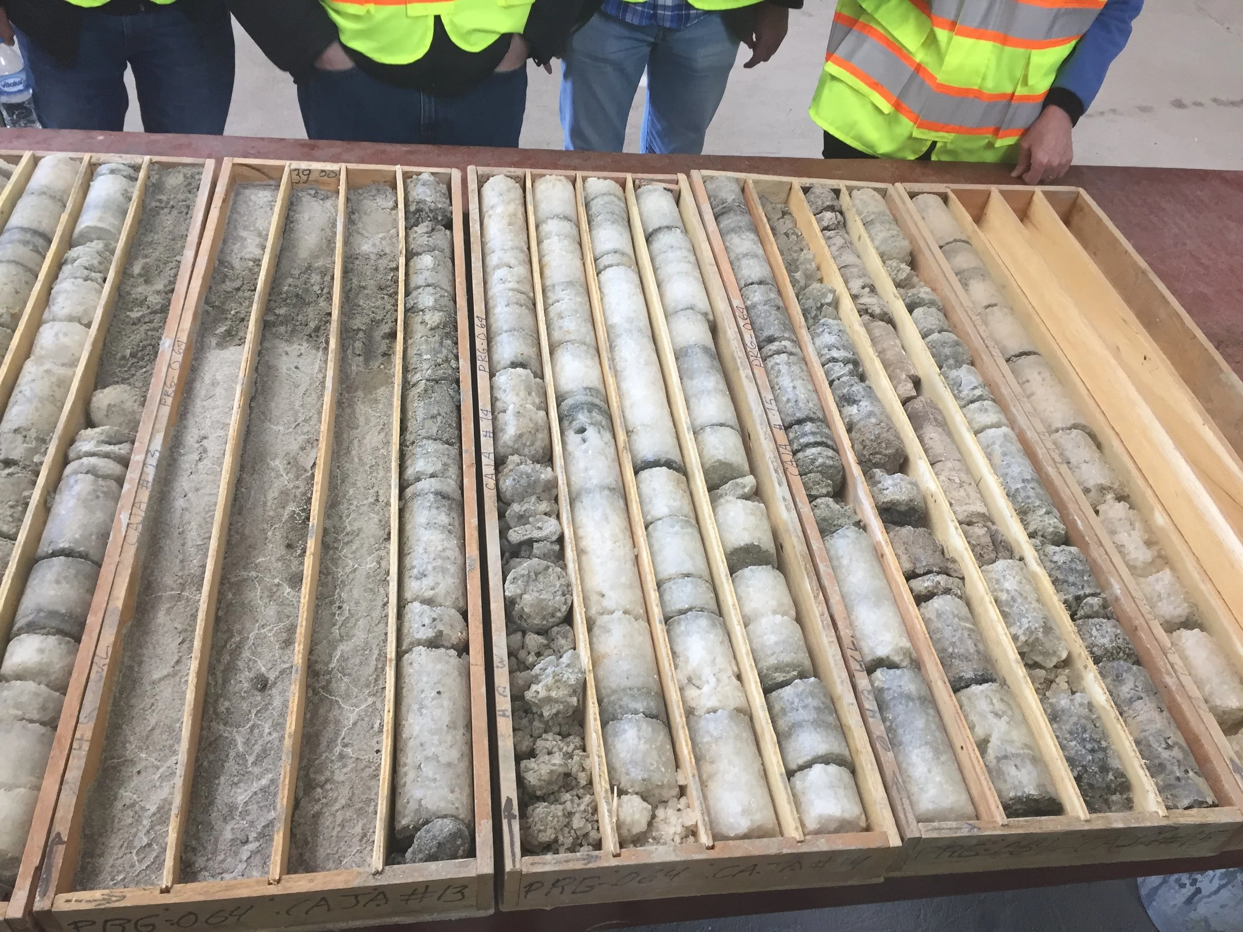
Drill core showing what looks like dull quartz - what could core scanning and machine learning reveal?

Modern core scanning equipment can capture optical photography, multispectral and hyperspectral imagery, portable XRF geochemistry, magnetic susceptibility measurements, and LiDAR surface data — all in a single automated pass. That is a remarkable volume of information from a single drill hole.

Most of it ends up on a hard drive, doing nothing.

And when companies do attempt to run machine learning on their core scan data, many make the same mistake: they put everything into the model.

It feels like the right call. More data, more context, better results. In practice, it tends to produce the opposite.

The Problem with More

Machine learning models for core scan classification are sensitive to data quality in ways that are easy to underestimate. Each sensor stream — optical, hyperspectral, pXRF, LiDAR — has its own uncertainty profile. Some streams are clean. Others are noisy. Feed a high-uncertainty stream into a model alongside a reliable one and the model tries to learn from both. The noise does not cancel out. It degrades the signal.

There is also the normalisation problem. Combining optical colour values with elemental concentrations with surface roughness measurements requires careful handling. Add more layers and the complexity multiplies. The computational overhead increases, the signal-to-noise ratio falls, and the model becomes harder to interpret and harder to trust.

This is not a theoretical concern. It is the most common failure mode in applied ML for mineral exploration: a technically capable team with good data and poor data selection. Getting data quality right before modelling is upstream of algorithm choice. The same principle applies at the feature level.

What Core Scanning Actually Produces

It helps to be specific about what you are working with, because each stream is suited to different questions.

Optical data captures wet and dry photography of the core surface. This is the geologist's primary visual reference, now at high resolution and consistent scale. Useful for broad lithological boundaries and sedimentary structures.

Multispectral and hyperspectral imaging records mineral spectra extending well beyond visible light into near-infrared and shortwave infrared. This is where alteration mineralogy becomes legible at a scale impossible to achieve by eye — clay minerals, carbonates, sulphates, and iron oxides all have diagnostic spectral signatures.

Portable XRF (pXRF) provides elemental geochemistry at centimetre-scale resolution. Strong for geochemical vectoring and grade proxies. Worth noting the precision limits: gold by pXRF is unreliable, and any grade predictions from pXRF data should be treated with appropriate scepticism until properly validated.

Magnetic susceptibility measures the magnetic properties of the rock, particularly useful for distinguishing mafic from felsic lithologies and for identifying magnetite-related alteration.

LiDAR records surface roughness. The standout application is geotechnical: distinguishing natural fractures from driller breaks objectively and consistently, at a scale that manual logging cannot match.

Each stream is valuable for specific questions. None is universally relevant. That distinction is the starting point for everything that follows.

Why Random Forest Works Well Here

For classification tasks on core scan data, Random Forest is usually the right starting point, for several practical reasons.

It is non-parametric: it does not assume input data follows any particular distribution. That matters because core scan data combines continuous measurements, spectral indices, and categorical geological variables — formats that do not naturally conform to the same statistical assumptions.

It handles class imbalance reasonably well. Most drill holes have far more of one lithology than another. A model trained on imbalanced classes will simply learn to predict the majority class. Random Forest has mechanisms to address this, though it is not immune and the issue needs monitoring.

The most useful feature, though, is variable importance ranking. After training, the model tells you how much each input contributed to the result. This is not just a diagnostic. It is geological feedback on your own assumptions.

If rubidium ranks low in a tungsten classification, that is the model telling you something about the geochemistry of the system. Remove it, retrain, and see what changes. This iterative loop between the model and the geological interpretation is where the real analytical value lives.

Build the Conceptual Model Before You Touch the Data

The single most important step in a core scan ML project is one that many teams skip: building a conceptual model before any data is selected.

The questions are not complicated. What are you trying to classify? Lithology, alteration zones, geotechnical domains, mineralised intervals? What geological process controls the boundaries you need to identify? What data streams are mechanistically linked to that process?

If you are mapping alteration zones in a porphyry copper system, hyperspectral data and pXRF are directly relevant. Alteration minerals have diagnostic spectral signatures and the geochemistry tracks the fluid pathways. LiDAR surface roughness is probably not relevant to that classification. Including it adds noise with no geological justification.

That seems obvious written down. It is surprisingly easy to skip when six sensor streams are available and the project timeline is tight.

The variable importance output from your first model run should feed directly back into this conceptual model. It will confirm some assumptions and challenge others. An input ranked unexpectedly low might be geologically irrelevant to your target. Or it might indicate poor data quality for that stream — calibration problems, spatial gaps, instrument inconsistency. That is a different problem with a different solution, and the distinction matters.

This is not a single-pass workflow. The model and the geological interpretation refine each other across multiple iterations. A willingness to revisit the conceptual model when the data says something unexpected is what separates useful ML from technically correct but geologically meaningless ML.

For a structured framework on evaluating ML robustness, the due diligence criteria for machine learning in mineral exploration are worth working through before you commit to a model design.

Uncertainty Is a Signal, Not a Failure

A classification map tells you what the model thinks each metre of core is. An uncertainty map tells you where the model is not sure. That second map is often more informative than the first.

High-uncertainty zones are worth investigating. The cause might be a lithology that is underrepresented in the training data. It might be an instrument gap — a section where calibration was inconsistent or a sensor malfunctioned. It might be a genuine geological boundary, where two units grade into each other and the classes are not as cleanly separable as the model assumes. Or it might be a fault zone, where intense fracturing produces a genuinely ambiguous signal.

A geologist reviewing the uncertainty map can usually distinguish these cases. Each has a different implication. Add more training samples. Improve calibration. Revisit the class definitions. Flag for structural interpretation.

Treating uncertainty as something to be minimised misses the point. It is a signal about the limits of the data and the model, and about the geology. Building a workflow that captures and interrogates it is as important as building one that produces accurate classifications.

Match Complexity to the Problem

Not every core scan problem needs the same approach, and overengineering is its own failure mode.

Simple binary classification — granite versus basalt — can often run on optical data alone. RGB colour change across the core is usually sufficient. Adding a full multi-sensor dataset increases complexity without improving the result.

Moderate complexity problems, like mapping alteration zones in a polymetallic system, typically benefit from combining pXRF and hyperspectral data. Random Forest handles this well with appropriate feature selection.

High-complexity problems — predicting gold grade at fine spatial resolution, or resolving subtle mineralogy in a deposit with complex paragenesis — may require convolutional neural networks or other deep learning approaches. These need substantially more training data, more computational resource, and more rigorous validation. They are not always justified. The deposit dictates the approach.

Machine learning in core scanning is not replacing geologists. The combination of geological expertise and data science expands what is possible at a scale and consistency that manual logging cannot match. But geological expertise is upstream of the model, not downstream of it. A model built without a conceptual foundation will find patterns. They will not necessarily be the patterns that matter.